Mastering mixture modeling
Mixture models (also known as "Scheffé," after the inventor) differ from standard polynomials by their lack of intercept and squared terms. For example, most of us learned about quadratic models in high school and/or college math classes, such as this one for two factors:
These models are extremely useful for optimizing processes via response surface methods (RSM) such as central composite designs (CCDs).
Mixture models look different. For example, consider this non-linear blending model for the melting point (Y) of copper (X₁) and gold (X₂) derived from a statistically designed mixture experiment*:
As you can see, this equation, set up to work with components coded on a 0 to 1 scale, does not include an intercept (ß₀) or squared terms (X₁², X₂²). However, it works quite well for predicting the behavior of a two-component mixture. The first-order coefficients, 1043 and 1072, are quite simple to interpret—these fitted values quantify the measured** melting points in degrees C for copper and gold, respectively. The difference of 29 characterizes the main-component effect (copper 29 degrees higher than gold).
The second-order coefficient of 536 is a bit trickier to interpret. It being negative characterizes the counterintuitive (other than for metallurgists) nonlinear depression of the melting point at a 50/50 composition of the metals. But be careful when quantifying the reduction in the melting: It is far less than you might think. Figure 1 tells the story.
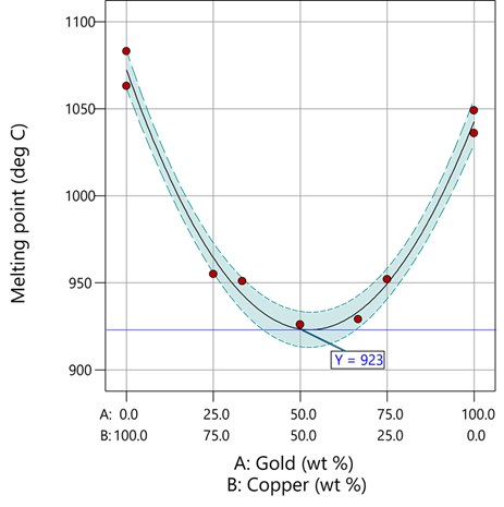
Figure 1: Response surface for melting point of copper versus gold
First off, notice that the left side—100% copper—is higher than the right side—100% gold. This is caused by the main-component effect. Then observe the big dip in the middle created by a significant, second-order impact from non-linear blending. Because of this, the melting point reaches a minimum of 923 degrees C at and just beyond the 50/50 blend point. This falls 134 degrees below the average melting point of 1057 degrees. Given the coefficient of -536 on the X₁X₂ term, you probably expected a much bigger reduction. It turns out 541 divided by 4 equals 134. This is not coincidental—at the 50/50 blend point the product of the coded values reaches a maximum of 0.25 (0.5 x 0.5), and thus the maximum deflection is one-fourth (1/4) of the coefficient.
If your head is spinning at this point, I advise you not to attempt to interpret coefficients of the mixture model beyond the main component effects and, if significant, only the sign of the second-order, non-linear blending term, that is, whether it is positive or negative. Then after validating your model via Stat-Ease software diagnostics, visualize the model performance via our program’s wonderful model graphics—trace plot, 2D contour, and 3D surface. Follow up by doing a numeric optimization to pinpoint an optimum blend that meets all your requirements.
However, if you would like to truly master mixture modeling, come to our next Fundamentals of Mixture DOE workshop.
* For the raw data, see Table 1-1 of A Primer on Mixture Design: What’s in it for Formulators. Due to a more precise fitting, the model coefficients shown in this blog differ slightly from those presented in the Primer.
** Keep in mind these are results from an experiment and thus subject to the accuracy and precision of the testing and the purity of the metals—the theoretical melting points for pure gold and copper are 1064 and 1085 degrees C, respectively.
Like the blog? Never miss a post - sign up for our blog post mailing list.