Gaussian Process Models (Stat-Ease 360^® only)

Introduction

Gaussian process models [RW06] are used in computer experiments, where instead of a physical or chemical process, the runs are evaluated using a simulation that may take a great deal of time. A Gaussian process model can be used as a surrogate for the simulation to make predictions or find optimal operating parameters when the data aren’t well fit by a polynomial. For a more in-depth study of computer experiments, see Santner et al. (2003) [SWN03].

Case Study: Gas Station

A convenience store chain wants to open a new gas station, and is trying to determine the number of pumps and the capacity of the underground storage tank required for the new store. Using a computer simulation, they are able to calculate the average wait time of vehicles throughout a typical day. However, the simulation is very computationally expensive to run, and so cannot be used with an optimizer.

The outputs of the simulator are the average wait time over the course of a day and the number of vehicles that abandon the queue due to an overly long wait.

Fewer pumps and a smaller tank are desirable to reduce the initial cost, as well as ongoing maintenance. The number of pumps directly impacts the number of vehicles that can be serviced at any given time. If the underground tank is too small it may need to be refilled during peak demand. This causes all pumping to pause while it is filled.

Latin Hypercube Design

Open Stat-Ease, and click on the Help, Tutorial Data menu and select Gas Station.

The vehicle simulator is deterministic. It will always result in the exact same average wait time and queue abandon rate given the same inputs. As such, a traditional designed experiment with replicates is inappropriate. Instead we will use a Latin Hypercube Design (LHD). This design has several properties that are desirable for a computer experiment:

1. It is a space-filling design.

2. It has no replicates.

3. The design resulting from removing a factor will also have no replicates (projection).

You’ll notice there is an additional response column for the cost of the station, which is an Equation Only response that we’ll use in optimization.

Click on the Custom Graphs node, then graph Pumps vs Tank Size. This plot demonstrates the space-filling properties of the LHD.

You may notice that there are replicates along the X axis, for example there are two tank sizes at 4 pumps. This is because a fraction of a fuel pump is nonsensical, so the Pumps factor was rounded and converted to a Discrete Numeric factor type. We’ve lost the projection property of the LHD, but this will allow us to restrict the predictions and optimization algorithm to integers.

Gaussian Process (Zero-Error) Analysis

Click on the avg wait time response to begin the analysis. Switch to Gaussian Process (Zero Error) in the Special Models dropdown and click Start Analysis.

The Factors tab allows you to remove a factor column from the analysis. In this case we’ll want to use both factors, so leave them alone. The Gaussian process kernel has a smoothing parameter that can be adjusted on this tab. For now we’ll leave the Select using setting at Maximum Likelihood. This selects the smoothing parameter optimally by maximizing the likelihood function for the Gaussian process. Press Calculate to see the estimate.

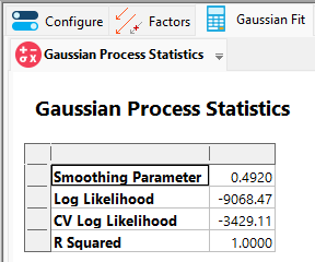
Next, click on the Gaussian Fit tab. Here you will find information about the Gaussian process regression, including the smoothing parameter and a coefficient of determination (R Squared) summarizing the fit.

Note

For zero-error Gaussian process regression the R Squared value will be 1 unless there are numerical problems or repeated factor combinations with different response values. Repeated factor combinations can occur when there are replicates in the design or when excluded factors result in repeated combinations in the remaining factors. If you would like to see this behavior for yourself, remove factor B-Tank Size and then click on the Gaussian Fit tab again.

Some groups of repeated values of A-Tanks are associated with different values for R1:avg weight time so the fit can’t be exact there, resulting in a R Squared value less than 1.

Don’t forget to add B-Tank Size back to the model before continuing with the tutorial.

After fitting a Gaussian process model for A-Tanks and B-Tank Size, click the Diagnostics tab for a graphical summary of predictions and raw residuals.

As expected, the residuals are small, and the predictions match the actual values very well. This is what is meant by “zero-error”; at the design points, the error should be consistent with rounding error and that is what the raw residual plots indicate.

Continue to the Model Graphs tab and switch to the 3D Surface plot.

The zero-error Gaussian process prediction surface matches the observed values with reasonable interpolation between the design points.

Repeat the above process for the R3:fraction abandoned response.

Gaussian Process (Noisy) Analysis

The zero-error Gaussian process models fit above are most useful for deterministic simulations – ones that give the exact same response outputs for the same factor inputs such as the Gas Station simulation discussed here.

By contrast, non-deterministic simulations include random error added to the response. Each run of the simulation results in a slightly different response value for the same inputs. Such simulations may be better fit, therefore, by a Gaussian process model that incorporates random noise.

We will take advantage of Stat-Ease software’s multiple analysis feature to create another analysis based on the average wait time data. Click on the Analysis [+] text above the existing response analyses. This will bring up the following dialog:

We want a new analysis based on R1: avg wait time, so leave the Response dropdown alone and click OK and then click the Rename button to the right of the Analysis name line. Type avg wait time - noisy GP for the new name and click OK.

Next, click on the Special Models radio button and select Gaussian Process (Noisy) from the dropdown.

Click Start Analysis to proceed to the Factors tab. Click Calculate. You will find that both a smoothing parameter and a noise parameter are reported for noisy Gaussian process models.

Click on the Gaussian Fit tab.

See the entry on Gaussian Process Models for more information on the various fields.

Next, click on the Model tab and then select the 3D plot to examine the predictive surface.

By relaxing the assumption of zero experimental error, the Gaussian process model is no longer constrained to fit exactly at the design points, resulting in a larger smoothing parameter. A larger smoothing parameter means a more slowly varying surface (fewer dimples or short-scale changes between observed values). In fact, the result is not dissimilar to what we would find if we fit a polynomial model to this data set (try this yourself!).

Because we know that this is a simulation with no experimental error, we will return to the zero-error Gaussian process model going forward.

Optimization

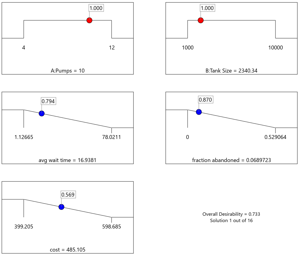
Now we are ready to find the optimal setup for the gas station. Go to the Numerical Optimization node. We’ll want to minimize the avg wait time and fraction abandoned responses, as well as the cost (which has the effect of minimizing both factors).

The optimizer finds a solution that is midway between the least and most expensive options. The average wait time of 17s is acceptable, and relatively few vehicles abandon the queue.

It would be reasonable to consider retaining as many vehicles as possible to be a greater priority than the wait time or cost. Stat-Ease has two ways to tweak the optimizer to better handle this important response. Go back to the Criteria tab, and you will see an Importance dropdown. Switch to the fraction abandoned criteria and see what setting this to +++++ does to the results.

Even with the higher importance we still get >5% abandoned.

Go back to the fraction abandoned criteria again and this time, grab the box in the middle of the criteria diagram and drag it to the bottom. This will modify the criteria so the desirability increases exponentially as you approach 0%. The same result can be achieved by increasing the Weights fields.

By increasing the number of pumps we’ve dropped the predicted abandon rate to 0.2%.

This corresponds to roughly 4 cars per day as opposed to 100, which will probably pay for the increased cost of the station over a period of time.

Finally, click on Graphs to verify that the solution maximizes the desirability by simultaneously minimizing the average wait time, fraction abandoned, and cost.

Extra Credit

You’ll notice that there is a column for the number of abandoned cars predicted by the simulator. This count response can be analyzed using Poisson regression as an alternate model to the fraction response. Try it out and see how the predictions differ. The simulation uses 2030 vehicles per day, so multiply the fraction response predictions by that to compare with the count.

References