Stat-Teaser April 2017

April 2017

In this issue:
1. Hear Ye, Hear Ye: An In-Class Response Surface Method (RSM) Experiment on Sound Produces Surprising Results by Mark Anderson
2. See Us at the CAMO Futures Conference, May 31–June 1, 2017 in Glasgow, Scotland
3. Get Up-to-Speed on DOE with Our Instructor-Led Workshops
4. Stat-Ease Webinar: Practical DOE—Tricks of the Trade
5. Thinking Outside the Box by Using Standard Error to Constrain Optimization by Pat Whitcomb 
6. Save the Date for the 7th European DOE User Meeting in Paris, France!

Hear Ye, Hear Ye: An In-Class Response Surface Method (RSM) Experiment on Sound Produces Surprising Results

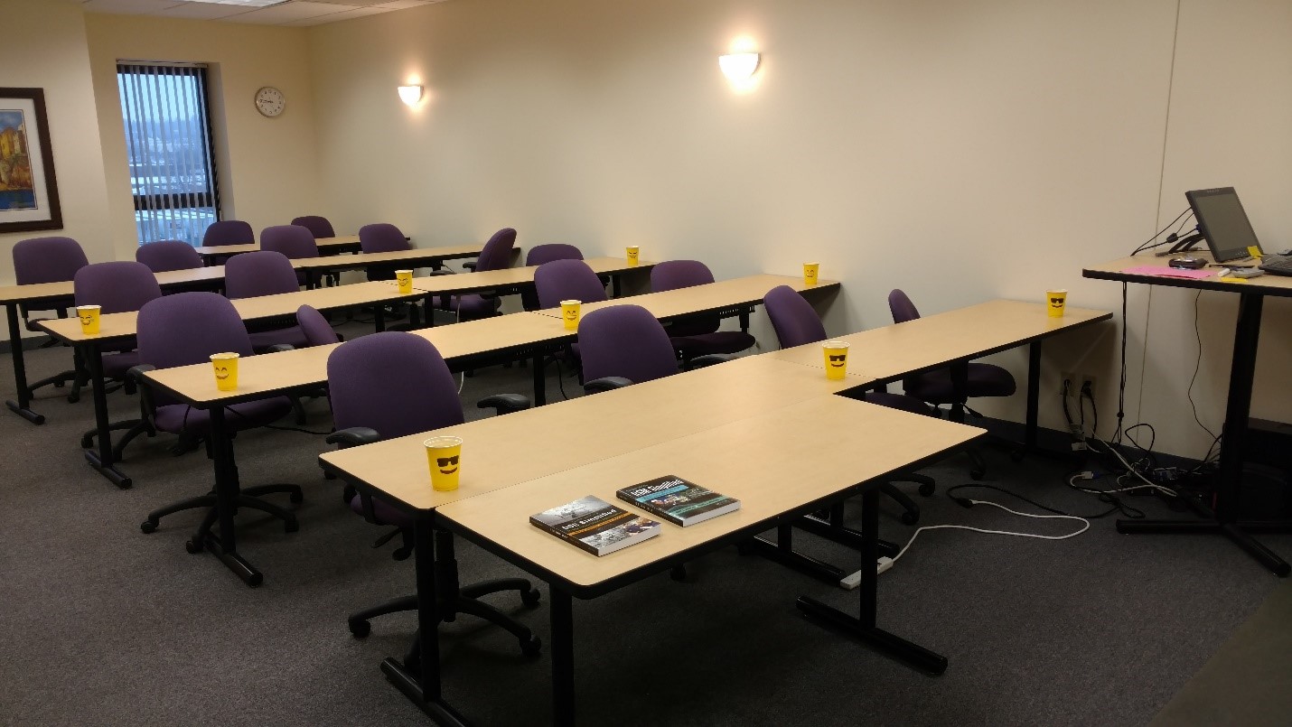
Stat-Ease training facility at Minneapolis headquarters—sound test points spotted by yellow cups

While developing our new DOE Simplified: Half-Day (DOESH) Workshop¹, I came up with a fun in-class experiment that demonstrates a great application of RSM for process optimization. It involves how sound travels to our students as a function of where they sit. The inspiration for this experiment came from a presentation by Tom Burns of Starkey Labs to our 5^th European DOE User Meeting. As I reported in our September 2014 Stat-Teaser, Tom put RSM to good use for optimizing hearing aids.²

Background

Classroom acoustics affect speech intelligibility and thus the quality of education. The sound intensity from a point source decays rapidly by distance according to the inverse square law. However, reflections and reverberations create variations by location for each student—some good (e.g., the Whispering Gallery at Chicago Museum of Science and Industry—a very delightful place to visit, preferably with young people in tow), but for others bad (e.g., echoing). Furthermore, it can be expected to change quite a bit from being empty versus fully occupied. (Our IT guy Mike, who moonlights as a sound-system tech, calls these—the audience, that is—“meat baffles”.)

Sound is measured on a logarithmic scale called “decibels” (dB). The dBA adjusts for varying sensitivities of the human ear.

Frequency is another aspect of sound that must be taken into account for acoustics. According to Wikipedia³, the typical adult male speaks at a fundamental frequency from 85 to 180 Hz. The range for a typical adult female is from 165 to 255 Hz.

Procedure

This experiment sampled sound on a 3x3 grid from left to right (L-R, coded -1 to +1) and front to back (F-B, -1 to +1)—see a picture of the training room above for location—according to a randomized RSM test plan. A quadratic model was fitted to the data, with its predictions then mapped to provide a picture of how sound travels in the classroom. The goal was to provide acoustics that deliver just enough loudness to those at the back without blasting the students sitting up front.

Using sticky notes as markers (labeled by coordinates), I laid out the grid in the Stat-Ease training room across the first 3 double-wide-table rows (4th row excluded) in two blocks:

1. 2² factorial (square perimeter points) with 2 center points (CPs).
2. Remainder of the 3² design (mid-points of edges) with 2 additional CPs.

I generated sound from the Online Tone Generator at 170 hertz—a frequency chosen to simulate voice at the overlap of male (lower) vs female ranges. Other settings were left at their defaults: mid-volume, sine wave. The sound was amplified by twin Dell 6-watt Harman-Kardon multimedia speakers, circa 1990s. They do not build them like this anymore. ; ) These speakers reside on a counter up front—spaced about a foot apart.  I measured sound intensity on the dBA scale with a GoerTek Digital Mini Sound Pressure Level Meter (~$18 via Amazon).

Results

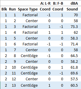
I generated my experiment via the Response Surface tab in Design-Expert^® software (this 3³ design shows up under "Miscellaneous" as Type "3-level factorial"). Via various manipulations of the layout (not too difficult), I divided the runs into the two blocks, within which I re-randomized the order. See the results tabulated below.

Table of results from the sound experiment

 

Notice that the readings at the center are consistently lower than around the edge of the three-table space. So, not surprisingly, the factorial model based on block 1 exhibits significant curvature (p<0.0001). That leads to making use of the second block of runs to fill out the RSM design in order to fit the quadratic model. I was hoping things would play out like this to provide a teaching point in our DOESH class—the value of an iterative strategy of experimentation.

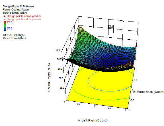
The 3D surface graph shown below illustrates the unexpected dampening (cancelling?) of sound at the middle of our Stat-Ease training room.

3D surface graph of sound by classroom coordinate

 

Perhaps this sound ‘map’ is typical of most classrooms. I suppose that it could be counteracted by putting acoustic reflectors overhead. However, the minimum loudness of 57.4 (found via numeric optimization and flagged over the surface pictured) is very hearable by my reckoning (having sat in that position when measuring the dBA). It falls within the green zone for OSHA’s decibel scale, as does the maximum of 73.6 dBA, so all is good.⁴

What next

The results documented here came from an empty classroom. I would like to do it again with students (aka meat baffles) present. I wonder how that will affect the sound map. Of course, many other factors could be tested. For example, Rachel from our Workshops team suggested I try elevating the speakers. Another issue is the frequency of sound emitted. Furthermore, the oscillation can be varied—sine, square, triangle and sawtooth waves could be tried. Other types of speakers would surely make a big difference.

What else can you think of to experiment on for sound measurement? Let me know.

—Mark J. Anderson, mark@statease.com

References

1. See www.statease.com/training/workshops/class-doesh.html for description and course outline, and www.statease.com/training/workshops.html for scheduling of public presentations. This, and any other workshop we offer, can be brought on site for a private class. For a quote, e-mail workshops@statease.com.
2. “Not listening in on what’s being said behind your back—DOE fine-tunes hearing aids” .
3. “Voice frequency” .
4. Figure 3, OSHA Technical Manual, Section III, Chapter 5: “Noise” .

↑Go back to the top

See Us at the CAMO Futures Conference, May 31–June 1, 2017 in Glasgow, Scotland

Stat-Ease's ally, CAMO Software, is holding their CAMO Futures conference this May 31–June 1 in Glasgow, Scotland.  It will focus on multivariate analysis and real-time process monitoring trends, insights, and networking. At the conference, Pat Whitcomb, President of Stat-Ease, will be speaking on "A Synergistic Blend of Multivariate Analysis Methods with Design of Experiments Tools" and Mark Anderson, Principal of Stat-Ease, will be teaching a pre-conference workshop on "DOE Simplified: Half-Day Workshop".  Registration is free for qualified attendees. If you are interested in attending this exciting conference, click here to learn more and register.  We hope to see you in Glasgow!

↑Go back to the top

Get Up-to-Speed on DOE with Our Instructor-Led Workshops

Whether you are just starting out with DOE or are a practiced experimenter, Stat-Ease has a workshop* for you. Our computer-intensive classes include hands-on exercises and one-on-one coaching by experienced instructors. Enroll at least 6 weeks prior to the date to assure your seat—plus get a 10% “early-bird” discount. Find a list of our upcoming public workshops below: 

• Designed Experiments for Pharma (DEPH)
• May 15-16, Edison, New Jersey (NJ)
• DOE Simplified: Half-Day Workshop (DOESH)
• May 19, Chicago, Illinois (IL)
• Modern DOE for Process Optimization (MDOE)
• June 20-22, Minneapolis, Minnesota (MN)
• Mixture and Combined Designs for Optimal Formulations (MIXC)
• July 18-20, Minneapolis, Minnesota (MN)

See this web page for complete schedule and site information on all Stat-Ease workshops open to the public. To enroll, scroll down to the workshop of your choice and click on it, e-mail workshops@statease.com, or call our Client Specialist Rachel Pollack, at 612-746-2030. If spots remain available, bring along several colleagues and take advantage of quantity discounts in tuition. Or, consider bringing in an expert from Stat-Ease to teach a private class at your site. Industry-specific classes are available. This is a cost-effective and convenient option if you have 6 or more people to train. For more information on private workshops, click here.

To view our e-learning options, see the Stat-Ease Academy. At your own pace, master the basics of statistics and how to apply DOE to maximum advantage. No traveling necessary! Some courses are available free of charge, while others can be purchased for a small fee.

*Workshops are limited to 16. Receive a $200 quantity discount per class when you enroll 2 or more students, or when a single student enrolls in multiple workshops. For more information, contact Rachel via e-mail or at at 612.746.2030.

↑Go back to the top

Stat-Ease Webinar: Practical DOE—Tricks of the Trade

 
Consultant Pat Whitcomb

Thinking Outside the Box by Using Standard Error to Constrain Optimization

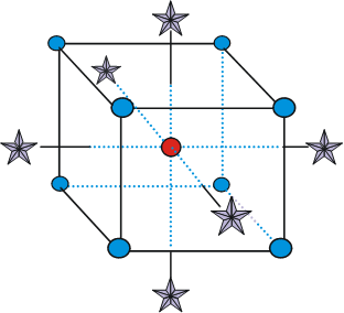
Response surface methods (RSM) pave the way to the pinnacle of process improvement. However, the central composite design (CCD)—the most common layout for RSM (pictured in Figure 1 for three factors)—traditionally limits the region of prediction to the cubical core. This conservative view avoids dangerous extrapolation out to the far corners of the space defined by the axial ranges of the star points. However, this can be very limiting, e.g., closing out the search even an iota outside the faces of the cubes. This article lays out a new, less-limiting (but still safe), approach to optimization based on using a specified standard error (SE) of prediction as the boundary for searching out the optimal process setup.

Figure 1: Central composite design for three factors

Three different methods for defining the search area will be detailed for a four-factor CCD. The goal is to avoid extrapolating beyond where the data provides adequate knowledge about the response, while maximizing the volume that will be explored. The breakthrough comes by making use of the SE of the predicted response mean, which at a point in the factor space (x_o) is:

where:

x₀ =  the location in the design space (i.e. the x coordinates for all model terms).

X =   the expanded design matrix (i.e. where the runs are in the factor space).

s =   the standard deviation measuring experimental error. For comparing the standard errors in the search areas a standard deviation of one is assumed, i.e. s=1.

Now let’s compare three boundaries for defining the search area in the factor space, the first two of which do not make use of the SE:

1. Factorial—the cube with vertices at coded values ±1.
   The volume of this four-dimensional hypercube is 16. The maximum SE is 0.764, which occurs at the vertices (i.e., corners). For comparison sake, figure on this SE (0.764) being the benchmark—anything more than this will be deemed unacceptable.
   
   
2. Axial—a cube with vertices at ±2 to include the star runs.
   The volume of this four-dimensional hypercube is huge: 256 coded units, which offers big advantages for optimization. However, the majority of the volume (69%) exhibits an SE ≥ 0.764 (maximum is 2.963!). Therefore, this method must be rejected.
   
   
3. Standard error—the area within SE ≤0.764.*
   For the 4-factor CCD the SE at the axial (star) points equals that of the ±1 factorial points. Limiting the standard error ≤0.764 produces a sphere with a radius of 2. Figures 2a and b show the 0.764 SE contours for two factors with the others fixed at zero (left) and +1 (right). The volume of this sphere is 78.96, almost five times larger than the ±1 factorial cube (shaded blue)!

Figures 2a, b: Two-factor standard error contours for a 4-factor CCD with the other factors at 0 and +1; respectively

Summarizing the three methods of defining the search area in the factor space:

1. The factorial cube with vertices at ±1 is too restrictive, it does not include all the volume of good predictions.
   
   
2. A cube with vertices at ±2 that includes the axial runs is too liberal—most of the volume has poor predictions.
   
   
3. Defining the search area by standard error is just right—it includes all the area of good predictions.

Using standard error to constrain the optimization defines a search area that matches its properties:

• Spheres for rotatable CCDs.
  
  
• Cubes for face centered CCDs.
  
  
• Irregular shapes for optimal designs and historical data.

An added bonus to using SE is that it adjusts the search area for reduced models and/or missing data.

For more details on this topic (and a couple of others), attend my upcoming webinar presented on June 12 and again on June 14 on “Practical DOE—Tricks of the Trade”.

Save the Date for the 7th European DOE User Meeting & Workshops in Paris, France!