Note
Screenshots may differ slightly depending on software version.
Combined Mixture-Process
Introduction
Stat-Ease® software offers designs that combine mixture components and process factors (numeric and/or categoric). In this tutorial, you will apply its unique features for mixture-process design and analysis by investigating John Cornell’s famous fish-patty experiment from his textbook Experiments with Mixtures, 3rd edition, published by John Wiley and Sons, New York. Zip through it all by skipping the sidebars, or, if you like to explore, take the time to study these.
Note
Before embarking on this tutorial, you should first complete the previous tutorial on mixture design.
P.S. Stat-Ease provides in-depth training on combined mixture-process in its Mixture Design for Optimal Formulations workshop. Call for information on content and schedules, or better yet, visit our web site at www.statease.com and click the “Learn DOE” link.
The food formulators hope to make something delicious from a blend of three tasty-sounding (?) fish: mullet, sheepshead, and croaker. Yum! The seven blends in the design include one each of the three fishes, plus three binary blends, and a blend of one-third each of the individual types of fish. The fish patties can be cooked at varying deep-frying time, oven temperature, and oven time. Combining each of these process factors at two levels for all seven blends creates a total of 56 experimental runs. The diagram below shows the blends as points on triangles, repeated at each of the eight corners of a cube representing the process.

Fish-patty design: Seven blends (on triangles) at eight process combinations (cube)
The response measure is patty texture. (Never mind about taste!)
The Experiment as Originally Run
Start the program and the quickest route to initiating a new design by clicking the New Design button on the opening screen.
Click Custom Designs to expand its menu and select the User Defined option. The user defined option allows you to reproduce Cornell’s design with all points chosen. Normally, to save on runs, you want to use the first choice on the list, Optimal, which selects an ideal subset of design points from a candidate set for a specified model. We’ll explore this option later.
For Mixture 1 Components, select 3 from the droplist. (Notice that Stat-Ease software offers the option for adding a second mixture, for example in a two-layer cake, film, or coating. For the number of Numeric Factors choose 3. Leave Categoric Factors at zero, but keep in mind for future experimentation that you can add discrete variables – such as who supplies a given component.

Specifying the combined user-defined design
Press Next and enter the Total for mixture components (fish types) at 100 and Units as %. Then enter fish names as shown below. Low limits remain zero. Set all high limits to 100.

Entering mixture details
Press Next to move on to the process factors. Enter their factor names, units, and ranges (low – L[1] and high – L[2]) as shown below.

Entering process details
Press Next to define the model you want to design for the combination of mixture and process variables in this experiment. The default model is quadratic by quadratic. Click the Edit model button and change the default for Process Order to Linear.

Specifying the design model for the mixture and process variables
Click the OK button to implement the change. Now, consider your “candidate” points. Normally only some of these points would actually make it to the design, but by choosing the User Defined option, you get all of them. However, there’s a problem—the Mixture candidate set of points (Mixture tab at upper-left screen box) contains more points than those chosen by Cornell. Fix this by clicking off Axial check blends, and Interior check blends. Only vertices, centers of edges, and overall centroid should now be checked. Press Calculate points to get a count — this subtotals to 7 for the mixture candidate points.

Candidate points for mixture
Now click the Process candidate points tab (right of Mixture tab). This design also contains more points than those chosen by Cornell, so click off every checkmark except Vertices.

Candidate points for the process
You should now see a subtotal of 8 process combinations, which combined with the 7 mixture candidates, generates 56 total runs (points).
Press Next to see the response specification form. Enter Ave Texture with units of gm*10^-3.

Entering response name and units
Press Finish to complete the design. Stat-Ease now displays the 56 experiments in random run order.
Analyze the Results
To view response data, click on the Help, Tutorial Data menu and select Fish Patties. Now click on the Design node on the left.
Look over all resulting response data: Results within the range of 2 to 3.5 are desirable.
To analyze the data, click the Analysis node labeled Ave Texture and press the Start Analysis button. Then click the Fit Summary tab. You now see a unique matrix of probabilities that helps you determine the best crossed model for mixture and process. As shown below, the software provides suggestion(s) on which combination is best—in this case, a quadratic (“Q”) mixture model crossed with a linear (“L”) process model.

Suggested model — quadratic (mixture) by linear (process)
Note
For a detailed explanation about how to interpret sequential p-values in this Fit Summary table for combined designs, see Stat-Ease’s Handbook for Experimenters (provided free of charge to all registered software users) section titled “Combined Mixture/Process Analysis Guide.” This section is available upon request to trial users.
Now click the Model tab atop your screen. Stat-Ease software uses the suggested model as its default. Accept this for the moment by clicking ahead to the ANOVA. Notice that many of the model terms, particularly ones of third-order (for example, ABF) exhibit high Prob>F values. This is a byproduct of crossing the two mixture and process models, which creates many superfluous higher-order terms. When analyzing designs like this, you will often find it beneficial to reduce your model to only the significant terms, subject to requirements for maintaining hierarchy (no interactions without their parent terms).

Initial ANOVA (no model reduction)
To reduce the model, go back to Model. You could manually deselect the insignificant terms observed from the ANOVA, but it is quicker to let Stat-Ease software do this for you. Click the Auto Select… button. Change the criterion to p-values. The statistical criterion is like the scoreboard for comparing the adequacy of alternative designs, here we’re comparing p-values. Next, change the selection mode to Backward.

Selecting p-values criterion and backward reduction for Auto Select…
This enables automatic model reduction by a backward (stepwise) algorithm. The default significance level (“Alpha”) for elimination is a probability value of 0.1. Click Start. You will be presented with a summary of the terms that were eliminated via the backward selection method. Click Accept to continue with the selected model. Then, click on the ANOVA to evaluate it (shown below). Note that all of the terms in the selected model have significant p-values values at the <0.05 alpha level.

Analysis of variance for reduced mixture-process model
The ANOVA table also shows that the reduced model produces a highly-significant F Value (p-value < 0.0001). Move over to the Fit Statistics pane (location will vary based on pane layout) — they look really good.

Fit statistics (with annotation)
Click the Diagnostics tab and examine the graphs of residuals.

Normal plot of residuals — looks good
The normal plot of residuals looks good, so move on to the Model Graphs to view the response in mixture (triangular) space (use blue layout icons to match layout in screenshot).

Model Graph with view of contour plot for mixture portion of combined design
Click or grab various process factors on the Graphs Tool and adjust them to see how response changes. For example, push all three bars to the right as shown below.

Process slide-bars pushed to their maximum levels
Notice by the hotter colors that texture increases at the 100 percent mullet (top of triangle).
Now right-click the Factors Tool where it shows D:oven temp and select X2 axis. As shown below, the view changes to process (rectangular) space.
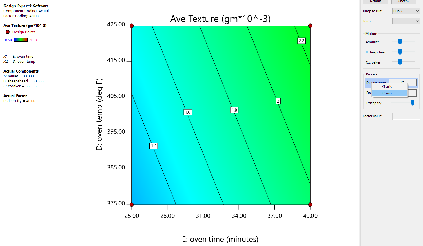
Changing to process view
Now shift back to mixture coordinates by right-clicking the Factors Tool where it lists A:mullet. Select X1 axis.

Back to mixture space
On the Graphs Toolbar click 3D Surface (may be offscreen to the right >>). Notice the strong tilt in the A-B axis.

3D mixture view
Press ahead to the 3D Surface Mix-Process display. It’s very likely you have never seen a plot like this!

3D plot of two mixture components versus one process factor!
Now you see the impact of shifting component A (mullet) in direct substitution for B (sheepshead) on one axis versus the process factor D (oven temp) on the other axis. Isn’t that something!
Continue if you like and explore different combinations of the mixture components and process factors in 2D contour view and 3D plots. Keep in mind that any textures outside of 2 to 3.5 are unacceptable.
Find the Optimal Solution
The goal of the experimental program is to learn how to produce fish patties with a texture in the range of 2.00 to 3.50 x 10⁻³ grams. The target is 2.75. To find optimal combinations of formulas and processing, click the optimization node labeled Numerical. Then select Ave Texture. Select a Goal of target-> and enter 2.75. For Limits enter a Lower of 2 and Upper of 3.5. Leave the weights and importance settings at their default levels. Your screen should now look like that below.

Optimization criteria for texture
Click the Solutions tab. If not already there by default, mouse to the Solutions Toolbar and select Ramps. Notice the many solutions listed in the solutions drop-down menu. (Due to the random nature of the optimization algorithm, your screen may show fewer or more solutions.) The software defaults to the most desirable solution.

One of many solutions for optimized texture (your results may vary)
Select solution number 2 and beyond: You will see many combinations that satisfy the texture requirements. Next press Graphs and you’re presented with the multiresponse graph showing the Desirability and Ave Texture graphs side by side. Select Desirability from the Response droplist on the solutions bar to focus on that response. Then, select 3D Surface from the Graphs Toolbar. Move your mouse cursor over the graph and when it turns into a hand (or crosshair) grab it by holding the left mouse button and rotate it to a vantage point like that shown below.

3D desirability view (your results may vary)
Note
Check out the desirability surface for other solutions. Remember that by right-clicking any of the process factors on the Factors Tool, you can create a graph in process space.
To preserve your modeling and optimization work, select File, Save or press
the ![]() icon.
icon.
The Experiment via Optimal Design
As noted in the introduction, we wanted to reproduce the fish patty case exactly as reported by Cornell in his textbook Experiments with Mixtures. Now let’s try an optimal design, which is much more efficient. We recommend you use this approach when designing your own mixture-process experiment. Assuming you are continuing from before, proceed by choosing File, New Design. The software asks whether to “Use previous design info?” Click Yes.

Re-using previous design information
You see the builder from the previous user-defined design session. Select Optimal (combined).

Optimal design option for combined mixture-process design
Press Next to see that all component names and Low/High values remain filled in for you. Press Next again to see your process factors, again at their previous ranges. Press Next one more time to bring up the Optimal Design screen. Notice it’s already set up for the quadratic-linear base model that you want for the fish-patties process-mixture design.
The objective of this exercise is to pick a subset of runs from Cornell’s actual experiment so the search must be limited to specific combinations – not just any coordinate within the mixture-process space. Therefore you must change the Search droplist from its default of “Best” to Point Exchange, as shown below.

Optimal design search by Point Exchange
Leave the optimality criterion at its default of “I” — a good choice in this case where continuous variables must be optimized. This criterion will dictate the selection of the minimal subset of model points from the candidate set, which in a moment you will specify as the original combinations run by Cornell.
Because the original data had no replicates, set Replicate points to 0. Hit the tab key and you see a total of 29 runs. Leave “Model points” and “To estimate lack of fit” at their default levels.

Default for replicates reduced to zero to match textbook case
Before continuing, you need to re-create the points originally selected by Cornell. (Recall doing this earlier when you set up the User Defined design.) Click Edit candidate points. In the Mixture 1 tab, check off Thirds of edges, Triple blends, Axial check blends, and Interior check blends. Press Calculate points. You now see a subtotal of 7 mixture points comprised of vertices (3), centers of edges (3) and the overall centroid (1). Go back to the screen shot shown on this earlier to be sure you have it right!
Next, press the Process tab and check off all points except for vertices. Click Calculate points. This produces a subtotal of 8 process points. You now have 56 total candidate points, the same as earlier when you set up this case study as a User Defined design.
Click OK and Next to move on to the response specification. Accept the default response name and units (as in the user defined example) by pressing Finish again.
Stat-Ease now builds the optimal design. Due to random elements in the algorithm (configurable via options), the 29 runs chosen may differ each time you do an optimal design, but they will be essentially identical in their matrix attributes.

Fish patty design: one possible subset of 29 I-optimal combinations
Remember that the point of this follow up to the first part of the tutorial is to show how you can get by with only a fraction of all possible mixture-process combinations by using an optimal design — in this case one that includes 29 combinations from within the original experiment, which contained 56 runs. Thus, this is a “what-if” exercise. If you were to build a completely new design for this case, it would be advisable to include the 5 replicates (34 total runs) that Stat-Ease suggests by default. This would provide 4 degrees of freedom to estimate pure error, which would allow a test for lack of fit, and generally improve the quality of the design. This subset is still much more efficient at fitting the specified model than the original 56 runs used by Cornell.
Note
As the number of mixture components and process factors increase, the runs required for traditionally crossed models become excessive. For that reason, newer versions of Stat-Ease software default to a “KCV” model. Learn more about this modern-DOE option via “Streamlined Models for Combined Mixture-Process Designs” by Pat Whitcomb—a March 2020 presentation.
Final comments
In all but the simplest cases, a User-Defined design (all possible combinations of mixture and process points) is too large to be practical. You will do well by using an optimal design, which provides a reasonable subset of points to estimate the model you specify. The KCV option (see note above) is most efficient by it estimating only the most likely first-order mixture-process interactions. If provided by your software, start with that as your first choice.
For any combined design, but especially if done via optimal for a minimum-run experiment, it’s advisable to override any suggested model that falls short of what can be estimated without aliases. When you analyze the results from a combined design, always try Stat-Ease software’s Auto Select. This model-reduction tool becomes more and more useful as the number of components and factors increase. You will see the payoff via the predicted R-squared—the best indicator of model fit.
