Note
Screenshots may differ slightly depending on software version.
Response Surface (pt 2)
Part 2/3 – Optimization
Introduction
This tutorial shows how to use Stat-Ease software for optimization experiments. It’s based on data from Response Surface Tutorial Part 1 - The Basics . You should go back to that tutorial if you have not completed it.
In this Response Surface Tutorial Part 2 - Optimization, you will work with predictive models for two responses, conversion and activity, as a function of three factors: time, temperature, and catalyst. These models are based on results from a central composite design (CCD) on a chemical reaction.
Use the Help, Tutorial Data menu and select Chemical Conversion (Analyzed) from the list.
To see an overview of the design, click the Summary node under the Design branch at the left of your screen. Then click the split-right view to see all three tables—Build Information, Factors and Responses.

Design summary
Now, for statistical details on the models, click on the Analysis Summary node at the bottom of the Post Analysis branch.

Analysis Summary
These tables provide convenient comparisons of the coefficients, fit statistics, model comparison statistics, and equations for all the responses.
Note
Because the Coefficients Table is laid in terms of coded factors you can make inferences about the relative effects. For instance, notice that the coefficient for AC (11.375) in the conversion equation is much higher than the coefficients for Factor B (4.04057). This shows, for the region studied, that the AC interaction influences conversion more than Factor B. The coefficients in the table are shadedby p-value, making it easy to see each term’s significance at a glance. In our example, we chose to use the full quadratic model. Therefore, some less significant terms (shown in gray) are retained, even though they are not significant at the 0.10 level.
P.S. Right-click any cell to export this report to PowerPoint or Word for your presentation or report. Check it out: This is very handy! Many other options become available by clicking the caret (v) to the right of the tab. Take a look!
Numerical Optimization
Numerical optimization will maximize, minimize, or target:
A single response
A single response, subject to upper and/or lower boundaries on other responses
Combinations of two or more responses.
Under the Optimization branch to the left of the screen, click the Numerical node to start.

Setting numerical optimization criteria
Setting the Optimization Criteria
The program allows you to set criteria for all variables, including factors and propagation of error (POE). (We will detail POE later.) It defaults factor ranges to factorial levels (plus one to minus one in coded values) — the region for which this experimental design provides the most precise predictions. Response limits default to observed extremes. In this case, you should leave the settings for time, temperature, and catalyst factors alone, but you will need to make some changes to the response criteria.
Now you get to the crucial phase of numerical optimization: assigning “Optimization Parameters.” The program uses five possibilities as a “Goal” to construct desirability indices (di):
Maximize,
Minimize,
Target->,
In range,
Equal to -> (factors only).
Desirabilities range from zero to one for any given response. The program combines individual desirabilities into a single number and then searches for the greatest overall desirability. A value of one represents the ideal case. A zero indicates that one or more responses fall outside desirable limits. The program uses an optimization method developed by Derringer and Suich, described by Myers, Montgomery and Anderson-Cook in Response Surface Methodology, 4th Edition, John Wiley and Sons, New York, 2016.
For this tutorial case study, assume you need to increase conversion. Click Conversion and set its Goal to maximize. As shown below, set Lower Limit to 80 (the lowest acceptable value), and Upper Limit to 100, the theoretical high.

Conversion criteria settings
You must provide both these thresholds so the desirability equation works properly. By default, thresholds will be set at the observed response range, in this case 51 to 97. By increasing the upper end for desirability to 100, we put in a ‘stretch’ for the maximization goal. Otherwise we may come up short of the potential optimum.
Now click the second response, Activity. Set its Goal to a target-> of 63. Enter Lower Limits and Upper Limits of 60 and 66, respectively. These limits indicate that it is most desirable to achieve the targeted value of 63, but values in the range of 60-66 are acceptable. Values outside that range are not acceptable.

Activity criteria settings
The above settings create the following desirability functions:
Conversion:
if less than 80%, desirability (di) equals zero
from 80 to 100%, di ramps up from zero to one
if over 100%, di equals one
Activity:
if less than 60, di equals zero
from 60 to 63, di ramps up from zero to one
from 63 to 66, di ramps back down to zero
if greater than 66, di equals zero
Note
Recall that at your fingertips you’ll find advice for using
sophisticated Stat-Ease software features by pressing the lightbulb (![]() ) button
to see Screen Tips on Numerical Optimization.
) button
to see Screen Tips on Numerical Optimization.
Changing Desirability Weights and the (Relative) Importance of Variables
You can select additional parameters called “weights” for each response. Weights give added emphasis to upper or lower bounds or emphasize target values. With a weight of 1, di varies from 0 to 1 in linear fashion. Weights greater than 1 (maximum weight is 10) give more emphasis to goals. Weights less than 1 (minimum weight is 0.1) give less emphasis to goals.
Note
Weights can be quickly changed by clicking and dragging the handles (squares ▫) on desirability ramps. Try pulling the square on the left down and the square on the right up as shown below.

Weights change by grabbing handles with mouse
This might reflect a situation where your customer says they want the targeted value (63), but if it must be missed due to a trade-off necessary for other specifications, it would be better to err to the high side. Before moving on from here, reenter the Lower and Upper Weights at their default values of 1 and 1; respectively. This straightens them to their original ‘tent’ shape.
“Importance” is a tool for changing relative priorities to achieve goals you establish for some or all variables. If you want to emphasize one over the rest, set its importance higher. Stat-Ease software offers five levels of importance ranging from 1 plus (+) to 5 plus (+++++). For this study, leave the Importance field at +++, a medium setting. By leaving all importance criteria at their defaults, no goals are favored over others.
Now click the Options button to see what you can control for the numerical optimization.

Optimization Options dialog box
Note
Click any particular option to get details. One that you should experiment with is the Duplicate Solution Filter, which establishes the minimum difference for eliminating essentially identical solutions. After doing your first search for the optimum, go back to this Option and change it one way and the other. Observe what happens to the solutions. If you increase it, you decrease the number. Conversely, reducing the value for the Filter increases the solutions.
Click OK to close Optimization Options.
Running the Optimization
Start the optimization by clicking the Solutions tab. It defaults to the Ramps view so you get a good visual on the best factor settings and the desirability of the predicted responses.

Numerical Optimization Ramps view for Solutions (Your results may differ)
The program randomly picks a set of conditions from which to start its search for desirable results – your results may differ. Multiple cycles improve the odds of finding multiple local optimums, some of which are higher in desirability than others. The program then sorts the results from most desirable to least. Due to random starting conditions, your results are likely to be slightly different from those in the report above.
Note
The ramp display combines individual graphs for easier interpretation. The colored dot on each ramp reflects the factor setting or response prediction for that solution. The height of the dot shows how desirable it is. View different solutions from the Solutions drop-down menu on the Factors tools; cycle through some of them and watch the dots. They may move only very slightly from one solution to the next. However, if you look closely at temperature, you should find two distinct optimums, the first few near 90 degrees; further down the solution list, others near 80 degrees.
The Solutions Toolbar provides three views of the same optimization. Click Report keeping in mind that the number of solutions you see will likely differ from what’s shown on the screenshot.

Report on numerical optimization
Now select the Bar Graph view from the Solutions Toolbar.

Solution to multiple response optimization — desirability bar graph
The bar graph shows how well each variable satisfies the criteria: values near one are good.
Optimization Graphs
Select the Graphs tab to view a contour graph of the overall desirability and all of your responses. On the Factors Tool palette, right-click C:Catalyst. Make it the X2 axis. Temperature then becomes a constant factor at 90 degrees (this level is picked automatically by the selected solution #1).

You can also use the droplist on the Graphs toolbar to look at bigger versions of each plot, such as the desirability plot below.

Desirability graph (after changing X2 axis to factor C)
The screen shot above is a graph displaying graduated colors – cool blue for lower desirability and warm yellow for higher.
The program sets a flag at the optimal point (as selected by the button bar at the top, number 1 is selected in the screenshot above). To view a response associated with the desirability, select the desired Response from its droplist. Take a look at the Conversion plot.

Conversion contour plot (with optimum flagged)
Note
Right-click over this graph and choose Graph Preferences. Then go to Surface Graphs and click Show 2D grid lines.

Show 2D grid lines option
Grid lines help locate the optimum, but for a more precise locator right-click the flag and Flag Size->Full to see the coordinates plus many more predicted outcome details. To get just what you want on the flag, right-click it again and select Edit Info.
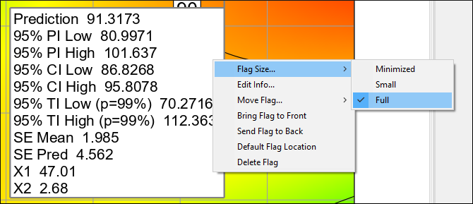
Flag size toggled to see select detail
To look at the desirability surface in three dimensions, again select Desirability from the Graphs toolbar drop-down. Then, press 3D Surface. Next, right-click the graph and select Set rotation and change horizontal control to 170. Press your Tab key or click the graph. What a spectacular view!

3D desirability plot
Now you can see there’s a ridge where desirability can be maintained at a high level over a range of catalyst levels. In other words, the solution is relatively robust to factor C.
Stat-Ease software offers a very high Graph resolution option. Right-click over your graph to bring up Graph preferences. Then, via the Surface Graphs tab change the 3D graph resolution to Very High.

3D graph resolution preference
However, you may find that the processing time taken to render this, particularly while rotating the 3D graph, can be a bit bothersome. This, of course, depends on the speed of your computer and the graphics card capability.
Now move on to graphical optimization. This may the best way to convey the outcome of a response surface method (RSM) experiment by displaying the “sweet spot” for process optimization.
Graphical Optimization
When you generated numerical optimization, you found an area of satisfactory solutions at a temperature of 90 degrees. To see a broader operating window, click the Graphical node. The requirements are essentially the same as in numerical optimization:
80 < Conversion
60 < Activity < 66
For the first response – Conversion (if not already entered), type in 80 for the Lower Limit. You need not enter a high limit for graphical optimization to function properly.

Graphical optimization: Conversion criteria
Click Activity response. If not already entered, type in 60 for the Lower Limit and 66 for the Upper Limit.
Now click the Graphs tab to produce the “overlay” plot. Notice that regions not meeting your specifications are shaded out, leaving (hopefully!) an operating window or “sweet spot.” Now go to the Factors Tool and right-click C:Catalyst. Make it the X2 axis. Temperature then becomes a constant factor at 90 degrees as before for Solution 1.

Overlay plot
Notice the flag remains planted at the optimum. That’s handy! This display may not look as fancy as 3D desirability, but it can be very useful to show windows of operability where requirements simultaneously meet critical properties. Shaded areas on the graphical optimization plot do not meet the selection criteria. The yellow “window” shows where you can set factors that satisfy requirements for both responses.
Note
Go back to the Criteria and click Use Interval (one-sided) for both Conversion and Activity. This provides a measure of uncertainty on the boundaries predicted by the models — a buffer of sorts.

Confidence intervals (CI) superimposed on operating window
After looking at this, go back and turn off the intervals to re-set the graph to the default settings.
P.S. If you are subject to FDA regulation and participate in their quality by design (QBD) initiative, the CI-bounded window can be considered to be a functional design space; that is, a safe operating region for any particular unit operation.
Let’s say someone wonders whether the 80 minimum for Conversion can be increased. What will this do to the operating window? Find out by dragging the 80 conversion contour until it reaches a value near 90. Then right-click it and Set contour value to 90 on the nose.

Changing the conversion specification to 90 minimum
It appears that the more ambitious goal of 90 percent conversion is feasible. This requirement change would make the lower activity specification superfluous as evidenced by it no longer being a limiting level; that is, not a boundary condition on the operating window.
Graphical optimization works great for two factors, but as factors increase, optimization becomes more and more tedious. You will find solutions much more quickly by using the numerical optimization feature. Then return to the graphical optimization and produce outputs at the various optimization solutions for exploration of the processing windows.
Response Prediction and Confirmation
This feature allows you to generate predicted response(s) for any set of factors. To see how this works, click on the Point Prediction node (lower left on your screen). Notice it now defaults to the first solution.

Point prediction set to solution #1
Confirmation
After finding the optimum settings based on your RSM models, the next step is to confirm that they actually work. To do this, click the Confirmation node (left side of your screen).

Confirmation predictions set to solution #1
Look at the 95% prediction interval (“PI low” to “PI high”) for the Activity response. This tells you what to expect for an individual (n = 1) confirmation test on this product attribute. You might be surprised at the level of variability, but it will help you manage expectations. (Note: block effects, in this case day-by-day, cannot be accounted for in the prediction.)
Of course you would not convince many people by doing only one confirmation run. Doing several would be better. For example, let’s say that the experimenters do three confirmatory tests. On the Confirmation Location #1 set Runs to 3 then press tab. You will now have 3 rows under Response Data, for Activity enter 62, 63 and 64.

Entering confirmation run results
Notice that the prediction interval (PI) narrows as n increases. Does the Data Mean (63) fall within this range? If so, the model is confirmed. If not, it will turn bold red.
Note
Keep increasing the value for n. Observe the diminishing returns in terms of the precision, that is, the PI approaches a limit — the confidence interval (CI) that you saw in Point Prediction. The CI is a function of the number of experimental runs from which the model is derived. That means one can only go so far with the number of confirmation runs – 6 may suffice.
Save the Data to a File
Now that you’ve invested all this time into setting up the optimization for this design, it would be prudent to save your work. If you are not worn out yet, you will need this file in Part 3 of this series of tutorials.
Summary
Numerical optimization becomes essential when you investigate many factors with many responses. It provides powerful insights when combined with graphical analysis. However, subject-matter knowledge is essential to success. For example, a naive user may define impossible optimization criteria that results in zero desirability everywhere! To avoid this, try setting broad acceptable ranges. Narrow them down as you gain knowledge about how changing factor levels affect the responses. Often, you will need to make more than one pass to find the “best” factor levels that satisfy constraints on several responses simultaneously.
This tutorial completes the basic introduction to doing RSM with Stat-Ease software. Move on to the next tutorial on advanced topics for more detailing of what the software can do.