Note
Screenshots may differ slightly depending on software version.
Historical Data
Part 1 – The Basics
Introduction
In this tutorial you will see how the regression tool in Stat-Ease® software, intended for response surface methods (RSM), is applied to historical data. We don’t recommend you work with such happenstance variables if there’s any possibility of performing a designed experiment. However, if you must, take advantage of how easy Stat-Ease makes it to develop predictive models and graph responses, as you will see by doing this tutorial. It is assumed that at this stage you’ve mastered many program features by completing preceding tutorials. At the very least you ought to first do the one-factor RSM tutorials, both part 1 and 2, prior to starting this one.
The historical data for this tutorial, shown below, comes from the U.S. Bureau of Labor Statistics via James Longley (An Appraisal of Least Squares Programs for the Electronic Computer from the Point of View of the User, Journal of the American Statistical Association, 62 (1967): 819-841). As discussed in RSM Simplified, 2nd ed. (Mark J. Anderson and Patrick J. Whitcomb, Productivity Press, New York, 2016: Chapter 2). It presents some interesting challenges for regression modeling.

Longley data on U.S. economy from 1947-1962
Assume the objective for analyzing this data is to predict future employment as a function of leading economic indicators – factors labeled A through F in the table above. Longley’s goal was different: He wanted to test regression software circa 1967 for round-off error due to highly correlated inputs. Will Stat-Ease be up to the challenge? We will see!
Let’s begin by setting up this “experiment” (quotes added to emphasize this is not really an experiment, but rather an after-the-fact analysis of happenstance data).
Design the “Experiment”
To save you typing time, we will re-build a previously saved design rather than entering it from scratch. Click on the Help, Tutorial Data menu and select Employment.
To re-build this design (and thus see how it was created), press the blank-sheet
icon (![]() ) at the left of the toolbar.
) at the left of the toolbar.

New Design icon
Click Yes when the program queries “Use previous design info?”

Re-using previous design
Click No when asked to save changes. Now you can see how this design was created via the Custom Designs tab and Blank Spreadsheet option.

Setting up blank spreadsheet design
Before moving ahead, you must set how many rows of data you want to type or copy/paste into the design layout. In this case there are 16 rows.
Press Next to view the factors. Note for each of the 6 numeric factors we entered name, units, and range from minimum (“Min”) to maximum (“Max”). Press Next to accept all entries on your screen.

Factor details
You now see response details – in this case only one response.

Response entry
Press Finish to see the resulting design layout in run order.
A Peculiarity on Pasting Data
Note
Consider taking a shortcut by simply pressing the Import Data button on the program’s opening screen (this option also appears under Custom Designs). Then follow the on-screen instructions to bring in your preexisting results straightaway—no need to first set up a blank spreadsheet: Much easier!
You could now type in all data for factor levels and resulting responses, row-by-row. (Don’t worry: we won’t make you do this!) However, in most cases data is already available via a spreadsheet. If so, simply click/drag these data, or copy to the clipboard, then Edit, Paste (or right-click and Paste as shown below) into the design layout. (Be sure, as shown below, to first select the top row of all your destination cells.)

Correct way to paste data into Stat-Ease (top-row of cells pre-selected)
If you simply click the upper left cell in the empty run sheet, the program only pastes one value.
Analyze the Results
Normally you’d save your work at this stage, but because we already did this, simply re-open our file: Click on the Help, Tutorial Data menu and select Employment. Click No to pass up the opportunity to save what you did previously.

Last chance to save (say “No” in this case)
Before we get started, be forewarned you will encounter many statistics related to least squares regression and analysis of variance (ANOVA). If you are coming into this without previous knowledge, pick up a copy of RSM Simplified and keep it handy. For a good guided tour of statistics for RSM analysis, attend our Stat-Ease workshop titled Modern DOE for Process Optimization.
Under the Analysis branch, click the Employment node. The program displays a screen for transforming response. However, as noted by the program, the response range in this case is so small that there is little advantage to applying any transformation.
Press the Start Analysis button to bring up the Fit Summary. The program evaluates each degree of the model from the mean on up. In this case, the best that can be done is linear. Anything higher is aliased.

Fit Summary – only the linear model is possible here
Move on by pressing Model.

Linear model is chosen
It’s all set up how the program suggested. Notice many two-factor interactions
can’t be estimated due to aliasing – symbolized by a yellow triangle with an
exclamation point ( ). Hold on to your hats (because this upcoming data
is really a lot of hot air!) and press ANOVA (analysis of variance).
). Hold on to your hats (because this upcoming data
is really a lot of hot air!) and press ANOVA (analysis of variance).

Analysis of variance (ANOVA)
Notice although the overall model is significant, some terms are not.
Note
Some statistical details on how |dex-name| does analysis of variance: You may have noticed this ANOVA is labeled “Sum of squares is Type III - Partial. This approach to ANOVA, done by default, causes total sums-of-squares (SS) for the terms to come up short of the overall model when analyzing data from a nonorthogonal array, such as historical data. If you want SS terms to add up to the model SS, go to Edit, Preferences for Analysis and change the default to Sequential (Type I) for these numeric factors. However, we do not recommend this approach because it favors the first term put into the model. For example, in this case, ANOVA by partial SS (Type III – the default of DX) for the response (employment total) calculates prob>F p-value for A as 0.8631 (F=0.031) as seen above, which is not significant. Recalculating ANOVA by sequential sum of squares (Type I) changes the p to <0.0001 (F=1876), which looks highly significant, but only because this term (main effect of factor A) is fit first. This simply is not correct.
Assuming Factor A (prices) is least significant of all as indicated by default ANOVA (partial SS), let’s see what happens with it removed. However, before we do, move to the Fit Statistics pane (shown below) to help us compare what happens before and after reducing the model.

Model statistics
Also look at the Coefficients estimates.

Coefficient estimates for linear model
Notice the huge VIF (variance inflation factor) values. A value of 1 is ideal (orthogonal), but a VIF below 10 is generally accepted. A VIF above 1000, such as factor B (GNP), indicates severe multicollinearity in the model coefficients (That’s bad!). In the follow-up tutorial (Part 2) based on this same Longley data, we delve more into this and other statistics generated by Stat-Ease for purposes of design evaluation. For now, right-click any VIF result to access context-sensitive Help, or go to Help on the main menu and search on this statistic. You will find some details there.
Press Model again. Double-click A-Prices to remove the “ ” (model)
designation and exclude the term.
” (model)
designation and exclude the term.

Excluding an insignificant term
You could now go back to ANOVA, look for the next least significant term, exclude it, and so on. However, this backward-elimination process can be performed automatically. Here’s how. First, reset Process Order to Linear.

Resetting model to linear
Now click on the Autoselect… button. Then change the selection to Backward and the Criterion to p-value.

Specifying backward regression
Notice a new field called “Alpha” appears. By default the program removes the least significant term, step-by-step, as long as it exceeds the risk level (symbolized by statisticians with the Greek letter alpha) of 0.1 (estimated by p-value). Let’s be a bit more conservative by changing Alpha to 0.05.
Now press the Start button to see what happens.
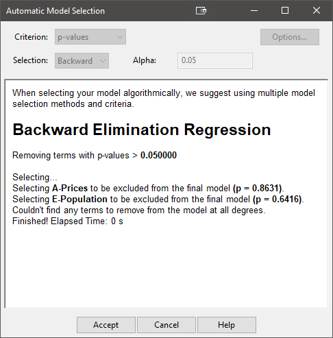
Backward regression results
The automatic selection is shown, step-by-step. Scroll up to see the whole thing if you like. For now, though, let’s move on and see what model is left and check out the more user friendly “selection log” to see what was done. The Start button becomes an Accept button, so click on that and then you click on the ANOVA to see the resulting model.

ANOVA for backward-reduced model
We are left with the same model we landed on by hand, but this was much easier. We also get a nice summary of how we got here. Click on the Model Selection Log pane.

Model Selection Log
Not surprisingly, the program first removed A and then E – that’s it. All of the other terms on the ANOVA table come out significant. (Note: If you do not see the report of the model being “significant” change your View to Annotated ANOVA.)
You may have noticed that in the full model, factor B had a much higher p-value than what’s shown above. This instability is typical of models based on historical data. Move over to the Fit Statistics and Coefficients panes.

Backward-reduced model statistics and coefficients
Now let’s try a different regression approach – building the model from the ground (mean) up, rather than tearing terms down from the top (all terms in chosen polynomial). Press Model, then re-set Process Order to Linear and click the Auto Select… button. This time choose p-values as your criterion and leave Forward for the Selection method. To provide a fair comparison of this forward approach with that done earlier going backward, change Alpha to 0.05.

Forward selection (remember to re-set model to the original process order first!)
Heed the text displayed by the program (When reducing your model…) because this approach may not work as well for this highly collinear set of factors. Press Start and then See what happens now in ANOVA.

Results of forward regression
Surprisingly, factor B now comes in first as the single most significant factor. Then comes factor C. That’s it! The next most significant factor evidently does not achieve the alpha-in significance threshold of p<0.05.
Move to the Fit Statistics pane.

Forward-reduced model statistics and coefficients
This simpler model scores very high on all measures of R-squared, but it falls a bit short of what was achieved in the model derived from the backward regression.
Finally, go back to Model, re-set Process Order to Linear and go to Autoselect… to try the last model Selection option offered by Stat-Ease: Stepwise (be sure to also choose p-value as your criterion). Note, AIC and BIC are newer model criterion that we will use in future tutorials.

Specifying stepwise regression
As you might infer from seeing both Alpha in and Alpha out now displayed, stepwise algorithms involve elements of forward selection with bits of backward added in for good measure. For details, search program Help, but consider this – terms that pass the alpha test in (via forward regression) may later (after further terms are added) become disposable according to the alpha test out (via backward selection). If this seems odd, look back at how factor B’s p-value changed depending on which other factors were chosen with it for modeling. To see what happens with this forward-selection method, press Start, Accept, and then ANOVA again. Results depend on what you do with Alpha in and Alpha out – both which default back to 0.1000. With the defaults, the same model is selected by this method as the backwards selection chose.
As you see in the message displayed for both forward and stepwise (in essence an enhancement of forward) approaches, we favor the backward approach if you decide to make use of an automated selection method. Ideally, an analyst is also a subject-matter expert, or such a person is readily accessible. Then they could do model reduction via the manual method filtered not only by the statistics, but also by simple common sense from someone with profound system knowledge.
Note
Consider preserving each alternative model for comparison via the Analysis [+] button in the tree on the left. This creates multiple analyses for any given response. Hint: To keep track of which is which, name each of your models in the field provided, for example, “p-value backward at 0.01”.
This concludes part 1 of our Longley data-set exploration. In Part 2 we mine deeper into Stat-Ease to see interesting residual analysis aspects within Diagnostics, and we also see what can be gleaned from its sophisticated tools within Design Evaluation.