Stat-Ease Blog

Categories
The Do's and Don'ts for Screening Process Factors
Adapted from Mark Anderson's 2023 webinar, "Do's & Don'ts for Screening Process Factors."
Over the years working with process development engineers on scale-up and manufacturing troubleshooting, we've noticed a pattern: the factors that experts think drive their process are rarely the whole story. There are often other variables at play that nobody anticipates. The best way to uncover these is by using screening designs: broad, shallow experiments that help you uncover previously unknown factors. Done right, a well-designed screening study can transform your understanding of a process and point you directly to the vital few factors worth exploring in depth.
First, let’s make sure we understand what a screening design does in the overall arc of process optimization. Screening designs exist to help ensure we are working with the right factors in subsequent optimization studies. Figure 1 explains the overall strategy. Note that interactions – often the key to process improvement – are not identified until the subsequent step. But a good screening design can shed some light on whether or not there are interactions to further pursue.
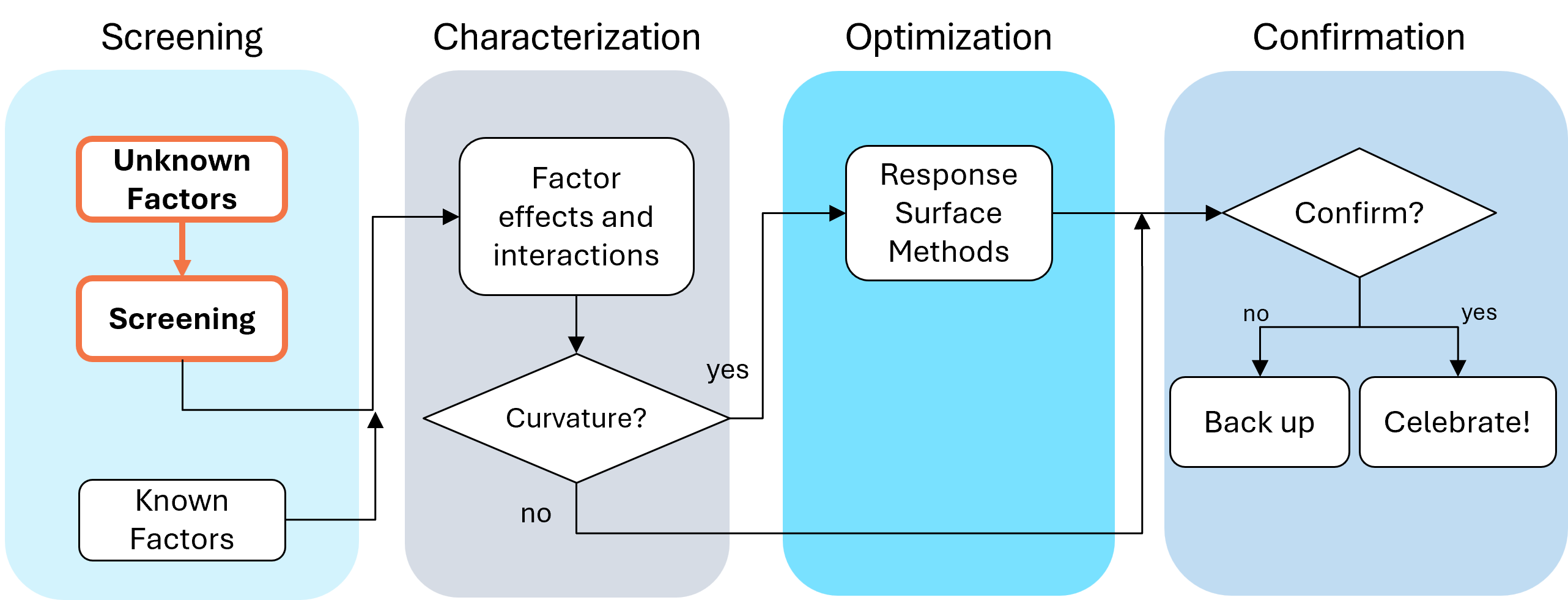
Fig. 1: Where screening fits in the SCOR strategy of experimentation.
With this strategy in view, here are the core do's and don'ts on screening designs. Consider this your field guide for avoiding the most common (and costly) mistakes.
DON'T: Include Factors You Already Know Will Affect the Process
This one surprises a lot of people, and has been the topic of heated discussions within our team. Why would you exclude a known important factor?
The answer is strategic focus and efficiency. By setting known factors aside during screening, you can concentrate on previously unknown factors: ones that might derail your process in unexpected ways. A broad and shallow two-level screening design lets you quickly identify the "vital few" from the "trivial many." In our experience, roughly 20% of factors you didn't expect to matter, matter! The known factors can be merged back in during the next phase of experimentation.
DON'T: Use Low Resolution Designs for Screening
This is our biggest pet peeve. Two types of designs fall into this trap: regular fractional factorials at Resolution III (shown as "red" designs in Stat-Ease software[MA3.1]), which alias main effects directly with two-factor interactions, and Plackett-Burman designs with even worse aliasing. That's a fatal flaw for screening, because if any factors interact (and in real processes, they often do) your main effect estimates are corrupted. You simply cannot trust what the analysis is telling you.
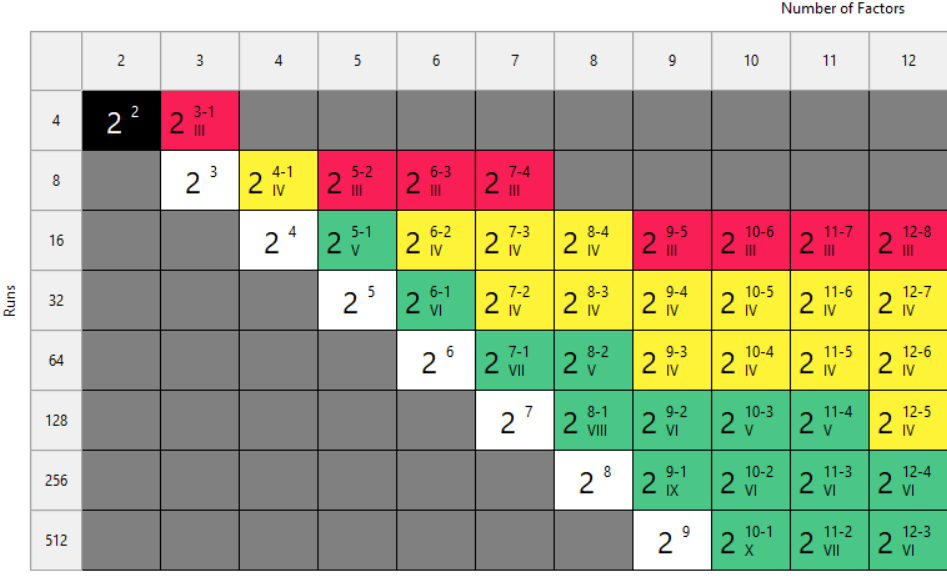
Fig. 2: Stat-Ease software's design picker, color-coded for your convenience.
We're particularly troubled by how often Plackett-Burman designs get recommended for screening. Even the NIST Engineering Statistics Handbook suggests using them, while simultaneously noting that “main effects are in general heavily confounded with two-factor interactions.” To us, that's an oxymoron. If main effects are confounded with two-factor interactions, how exactly is this a screening design? You can’t screen anything out!
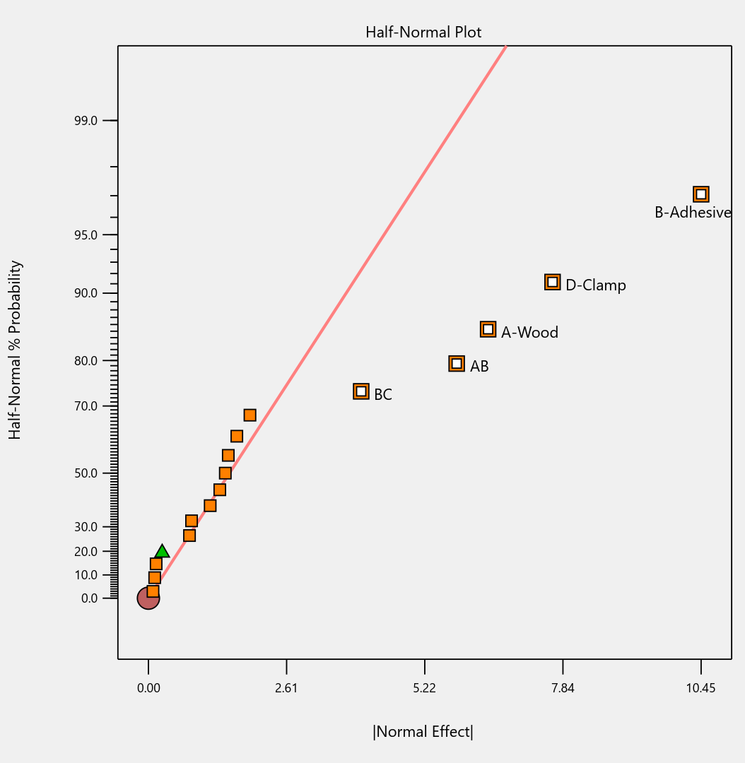
To illustrate the danger, we ran a simulation using the classic filtration rate dataset from Doug Montgomery's textbook Design and Analysis of Experiments. The full factorial result was clear: factors A (temperature), C (concentration), and D (stirring rate) were significant, along with strong AC and AD interactions.
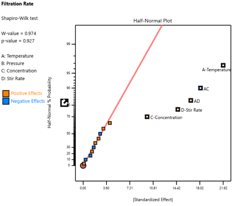
Fig. 3: Half-normal plot of effects for the full factorial design. Note that the selected effects are to well the right of the guideline.
When we re-ran the same underlying model through a 12-run Plackett-Burman simulation, the results were alarming. The AC and AD interactions got “smeared out” across multiple dummy factors. In particular, a fake factor E appeared significant when it was actually picking up aliased pieces of AC and AD. Meanwhile, the real main effect of D was undercut by its aliasing with one-third of AC, causing a cancellation. The result? Only factor A was correctly identified. Factors C and D were missed entirely.
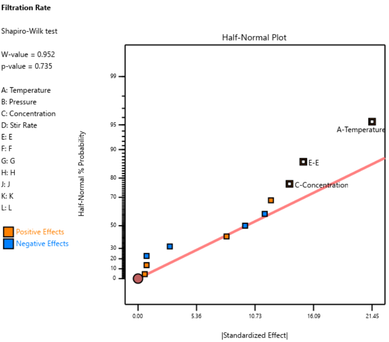
Fig. 4: Half-normal plot of effects for the Plackett-Burman design. None of the effects are to the right of the line, meaning this experiment shows no significant factors or interactions.
DOE pioneer George Box once said that running Resolution III or PB designs are "like kicking the TV to make it work." Sometimes you're desperate enough to try it, but there’s no guarantee you’ll get a usable result.
A Case Study in What NOT to Do
One of our users, a pharmaceutical process developer, sent in his design results hoping we could help salvage them. He had seven factors (time, temperature, and related process variables) and chose a Resolution III design with seven factors in eight runs. This is known as a ‘saturated’ design—the most factors that can be crammed into a given number of runs in a regular fractional factorial. Then, apparently recognizing the power would be low, he replicated the design, giving him 16 runs total, still at Resolution III.
As Ronald Fisher put it, a statistician is more like a pathologist than a medical doctor. We can tell you what killed the patient, but we can't bring it back to life. We wish this researcher had contacted us before running the design. The 16-run Resolution IV option for seven factors was right there in the software, highlighted in yellow (indicating a design more suitable for screening) It would have given him both the power and the resolution he needed. Instead, he replicated a bad design, which is a bit like making a photocopy of a photocopy.
The power calculations for these two designs are the clincher. One replicate of eight runs gave only 50% power to detect his specified signal-to-noise ratio of 1.67. Two replicates (still Resolution III) pushed that to about 87%: good power, terrible resolution. The unreplicated Resolution IV design in 16 runs also reached about 83% power, while giving him a design that could actually distinguish main effects from interactions.
DO: Start with a Resolution IV Design
As stated above, Resolution IV is the “Goldilocks” choice for screening. Main effects are aliased only with three-factor interactions, which are rarely active. That means that any significant main effects detected are almost certainly real. While two-factor interactions in a Res IV design may be murky, you'll know to investigate these further.
In Stat-Ease software, these are the yellow designs in the Regular Two-Level design builder. For up to eight factors, these medium resolution designs work beautifully. For nine or more factors, Stat-Ease’s proprietary, optimally templated, Minimum-Run screening design provides an excellent option when the standard design alternatives get too big.
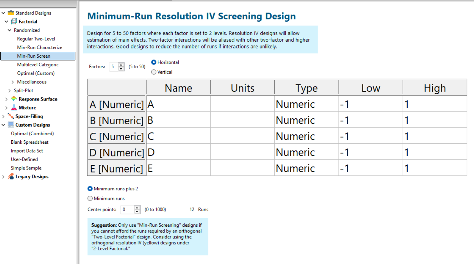
Fig. 5: Min-Run Screening designs in Stat-Ease software. Choose them from the sidebar on the left.
Summary: The Screening Do's and Don'ts
To recap: hold known factors aside during screening and focus on the unknowns. Known factors will be studied together with the survivors of the screening design in the next round of experimentation when characterizing two-factor interactions with high-resolution designs. Avoid low-resolution designs: the red standard ones or Plackett-Burmans. Instead, go with medium Resolution IV or minimum run screening design from the start.
All Stat-Ease software licensees have access to our DOE experts. We encourage you to contact us before making a big mistake in your design of experiments. Don’t hesitate to reach out: do your screening right the first time.
Like the blog? Never miss a post - sign up for our blog post mailing list.
10 highly intelligent features that make the most from every experiment
Stat-Ease software provides powerful tools for design of experiments (DOE) with a great deal of intelligence baked in. Here are 10 “smart” features that make DOE easy for our users. From bottom to top (ordered by DOE phase: design, modeling, optimization, and confirmation), every one of them provides great value.
Here we go—the countdown begins!
- Factorial design-building wizard guides you to right-sized experiments via a ‘heads-up’ on power to detect important effects despite the variability of run, sample, and test.
- Optimal design builder’s exchange algorithm delivers a finely crafted experiment customized per your specifications.
- Preset lineup of near-zero effects on the half-normal graph of factorial effects makes it easy to see those that merit selection.
- Scoring system for polynomial models suggests just the right 'Goldilocks' level that does not underfit or overfit your results.
- Box-Cox plot studies your model residuals and recommends whether or not to apply a transformation for a better fit and advises which one will do best.
- Detection of non-hierarchical models and, if you agree to fix this, the needed terms get added back for a well-formulated polynomial.
- Application of a curvature test to two-level factorial designs with center points with advice on how to augment the design if significant.
- Annotations on statistical outputs that explain them in plain English and provide advice on what to do when they go awry.
- Numerical search using a highly effective variable-size simplex algorithm finds the most desirable combination of factor settings and/or component levels meeting all your goals for process efficiency, product efficacy, and cost reduction.
- Confirmation tool smartly updates the prediction interval based on the number of follow-up runs at your chosen setting.
Finally, one bonus feature in Stat-Ease software that will make you more intelligent: screen tips via the lightbulb icon (click the >> chevron if showing) next to the Help bubble. This will show interesting information about each feature on the screen for you to understand the underlying statistics.
Email me your favorite “they thought of everything” quality aspect of Stat-Ease software, and I will add it to my list for my next ‘shout out’ on intelligent features.
August Publication Roundup
Here's the latest Publication Roundup! In these monthly posts, we'll feature recent papers that cited Design-Expert® or Stat-Ease® 360 software. Please submit your paper to us if you haven't seen it featured yet!
Featured Article
Design and optimization of imageable microspheres for locoregional cancer therapy
Scientific Reports volume 15, Article number: 27487 (2025)
Authors: Brenna Kettlewell, Andrea Armstrong, Kirill Levin, Riad Salem, Edward Kim, Robert J. Lewandowski, Alexander Loizides, Robert J. Abraham, Daniel Boyd
Mark's comments: This is a great application of mixture design for optimal formulation of a medical-grade glass. The researchers used Stat-Ease software tools to improve the properties of microspheres to an extent that their use can be extended to cancers beyond the current application to those located in the liver. Well done!
Be sure to check out this important study, and the other research listed below!
More new publications from August
- Use of experimental design for screening and optimization of variables influencing photocatalytic degradation of pollutants in aqueous media: A review of chemometrics tools
Chemical Engineering Research and Design, Volume 220, August 2025, Pages 270-291
Authors: Pedro César Quero–Jiménez, Aracely Hernández–Ramírez, Jorge Luis Guzmán–Mar, Jorge Basilio de la Torre–López, Matheus Silva–Gigante, Laura Hinojosa–Reyes - Analytical Quality by Design-Based Stability-Indicating UHPLC Method for Determination of Inavolisib in Bulk and Formulation
Separation Science Plus, no. 8 (2025): 8, e70110
Authors: Ashwinkumar Matta, Raja Sundararajan - Enhanced anti-infective activities of sinapic acid through nebulization of lyophilized protransferosomes
Frontiers in Nanotechnology | Biomedical Nanotechnology, Volume 7 - 2025
Authors: Hani A. Alhadrami, Amr Gamal, Ngozi Amaeze, Ahmed M. Sayed, Mostafa E. Rateb, and Demiana M. Naguib - Optimizing Anti-Corrosive Properties of Polyester Powder Coatings Through Montmorillonite-Based Nanoclay Additive and Film Thickness
Corrosion and Materials Degradation, 2025, 6(3), 39
Authors: Marshall Shuai Yang, Chengqian Xian, Jian Chen, Yolanda Susanne Hedberg, James Joseph Noël - Regulatory mechanism and multi-index coordinated optimization of pipeline transportation performance of coarse-grained gangue slurry: Experimental and simulation investigation
Physics of Fluids 37, 073343 (2025)
Authors: Jianfei Xu (许健飞); Jixiong Zhang (张吉雄); Nan Zhou (周楠); Hao Yan (闫浩); Wenfu Zhou (周文福); Qian Chen (陈乾); Jiarun Chen (陈嘉润) - Optimization of clayey soil parameters with aeolian sand through response surface methodology and a desirability function
Scientific Reports volume 15, Article number: 30831 (2025)
Authors: Ghania Boukhatem, Messaouda Bencheikh, Mohammed Benzerara, Mehmet Serkan Kırgız, N. Nagaprasad, Krishnaraj Ramaswamy, Souhila Rehab-Bekkouche, R. Shanmugam - Development of electromagnetic drop weight release mechanism for human occupied vehicle
Scientific Reports volume 15, Article number: 30663 (2025)
Authors: Sathia Narayanan Dharmaraj, Karthikeyan Shanmugam, Jothi Chithiravel, Ramesh Sethuraman - Operating parameter optimization and experiment of spiral outer grooved wheel seed metering device based on discrete element method
Scientific Reports volume 15, Article number: 30762 (2025)
Authors: Tao Zhang, Xinglong Tang, Cong Dai, Guiying Ren - Parameter optimization of key components in seed-metering device for pre-cut seed stems of Pennisetum hydridum
Scientific Reports volume 15, Article number: 31318 (2025)
Authors: Chong Liu, Xiongfei Chen, Qiang Xiong, Muhua Liu, Junan Liu, Jiajia Yu, Peng Fang, Yihan Zhou, Chuanhong Zhan, Yao Xiao - Optimization of new and thermally aged natural monoesters blends for a sustainable management of power transformers
Industrial Crops and Products, Volume 235, 1 November 2025, 121741
Authors: Gerard Ombick Boyekong, Gabriel Ekemb, Emeric Tchamdjio Nkouetcha, Ghislain Mengata Mengounou, Adolphe Moukengue Imano
Know the SCOR for a winning strategy of experiments
Observing process improvement teams at Imperial Chemical Industries in the late 1940s George Box, the prime mover for response surface methods (RSM), realized that as a practical matter, statistical plans for experimentation must be very flexible and allow for a series of iterations. Box and other industrial statisticians continued to hone the strategy of experimentation to the point where it became standard practice for stats-savvy industrial researchers.
Via their Management and Technology Center (sadly, now defunct), Du Pont then trained legions of engineers, scientists, and quality professionals on a “Strategy of Experimentation” called “SCO” for its sequence of screening, characterization and optimization. This now-proven SCO strategy of experimentation, illustrated in the flow chart below, begins with fractional two-level designs to screen for previous unknown factors. During this initial phase, experimenters seek to discover the vital few factors that create statistically significant effects of practical importance for the goal of process improvement.

The ideal DOE for screening resolves main effects free of any two-factor interactions (2FI’s) in broad and shallow two-level factorial design. I recommend the “resolution IV” choices color-coded yellow on our “Regular Two-Level” builder (shown below). To get a handy (pun intended) primer on resolution, watch at least the first part of this Institute of Quality and Reliability YouTube video on Fractional Factorial Designs, Confounding and Resolution Codes.
If you would like to screen more than 8 factors, choose one of our unique “Min-Run Screen” designs. However, I advise you accept the program default to add 2 runs and make the experiment less susceptible to botched runs.

Stat-Ease® 360 and Design-Expert® software conveniently color-code and label different designs.
After throwing the trivial many factors off to the side (preferably by holding them fixed or blocking them out), the experimental program enters the characterization phase (the “C”) where interactions become evident. This requires a higher-resolution of V or better (green Regular Two-Level or Min-Run Characterization), or possibly full (white) two-level factorial designs. Also, add center points at this stage so curvature can be detected.
If you encounter significant curvature (per the very informative test provided in our software), use our design tools to augment your factorial design into a central composite for response surface methods (RSM). You then enter the optimization phase (the “O”).
However, if curvature is of no concern, skip to ruggedness (the “R” that finalizes the “SCOR”) and, hopefully, confirm with a low resolution (red) two-level design or a Plackett-Burman design (found under “Miscellaneous” in the “Factorial” section). Ideally you then find that your improved process can withstand field conditions. If not, then you will need to go back up to the beginning for a do-over.
The SCOR strategy, with some modification due to the nature of mixture DOE, works equally well for developing product formulations as it does for process improvement. For background, see my October 2022 blog on Strategy of Experiments for Formulations: Try Screening First!
Stat-Ease provides all the tools and training needed to deploy the SCOR strategy of experiments. For more details, watch my January webinar on YouTube. Then to master it, attend our Modern DOE for Process Optimization workshop.
Know the SCOR for a winning strategy of experiments!
Augmenting One-Factor-at-a-Time Data to Build a DOE
I am often asked if the results from one-factor-at-a-time (OFAT) studies can be used as a basis for a designed experiment. They can! This augmentation starts by picturing how the current data is laid out, and then adding runs to fill out either a factorial or response surface design space.
One way of testing multiple factors is to choose a starting point and then change the factor level in the direction of interest (Figure 1 – green dots). This is often done one variable at a time “to keep things simple”. This data can confirm an improvement in the response when any of the factors are changed individually. However, it does not tell you if making changes to multiple factors at the same time will improve the response due to synergistic interactions. With today’s complex processes, the one-factor-at-a-time experiment is likely to provide insufficient information.
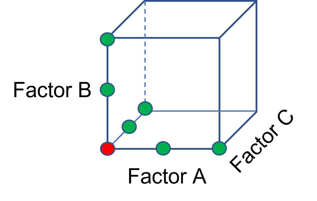
Figure 1: OFAT
The experimenter can augment the existing data by extending a factorial box/cube from the OFAT runs and completing the design by running the corner combinations of the factor levels (Figure 2 – blue dots). When analyzing this data together, the interactions become clear, and the design space is more fully explored.
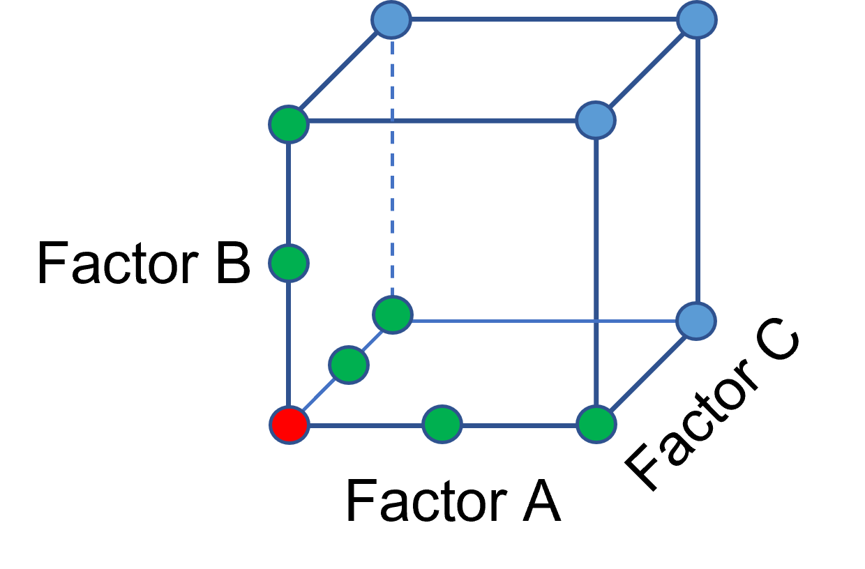
Figure 2: Fill out to factorial region
In other cases, OFAT studies may be done by taking a standard process condition as a starting point and then testing factors at new levels both lower and higher than the standard condition (see Figure 3). This data can estimate linear and nonlinear effects of changing each factor individually. Again, it cannot estimate any interactions between the factors. This means that if the process optimum is anywhere other than exactly on the lines, it cannot be predicted. Data that more fully covers the design space is required.
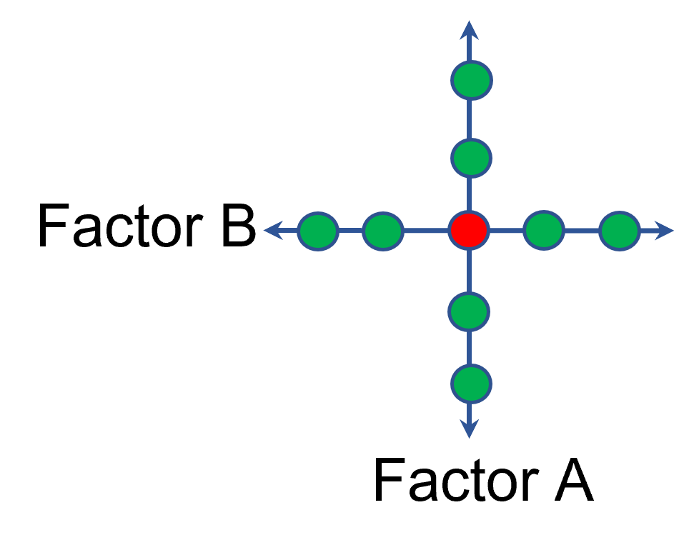
Figure 3: OFAT
A face-centered central composite design (CCD)—a response surface method (RSM)—has factorial (corner) points that define the region of interest (see Figure 4 – added blue dots). These points are used to estimate the linear and the interaction effects for the factors. The center point and mid points of the edges are used to estimate nonlinear (squared) terms.
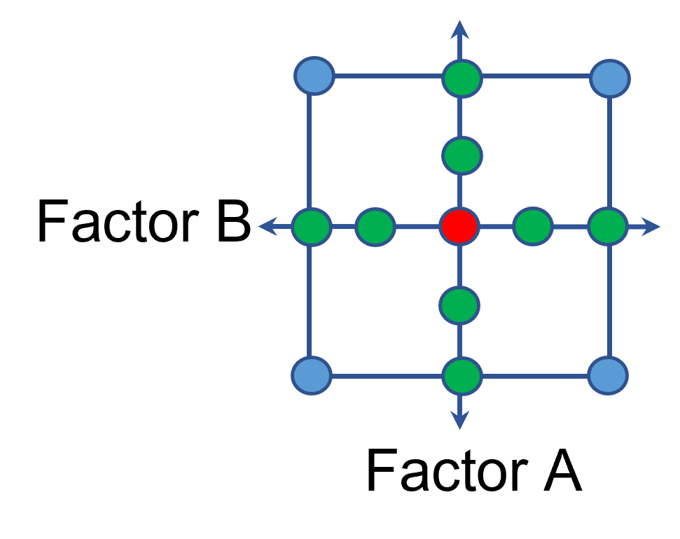
Figure 4: Face-Centered CCD
If an experimenter has completed the OFAT portion of the design, they can augment the existing data by adding the corner points and then analyzing as a full response surface design. This set of data can now estimate up to the full quadratic polynomial. There will likely be extra points from the original OFAT runs, which although not needed for model estimation, do help reduce the standard error of the predictions.
Running a statistically designed experiment from the start will reduce the overall experimental resources. But it is good to recognize that existing data can be augmented to gain valuable insights!
Learn more about design augmentation at the January webinar: The Art of Augmentation – Adding Runs to Existing Designs.